Exercise 02 solutions
🔹 must know, 🔸 ideally should know, ⛑ challenging, 🔫 very challenging
Exercise from Rasmus’ note
🔸 Exercise 1
Exercise 1. Find \(A\) and \(\mathbf{b}\) such that the system of equations below can be represented as \(A \mathbf{x}=\mathbf{b}\), compute the inverse of \(A\) and use it to find the solution.
\[\begin{array}{r} x+y+z=1 \\ 3 x+5 y+4 z=2 \\ 3 x+6 y+5 z=3 \end{array}\]Solution (based on Rasmus’ solution)
Let’s start by finding \(A\) and \(b\). Since the system is already in the nicely organized form, i.e. variables on the left side and constants on the right, we can simply rewrite the left side to the matrix form (\(A\)):
\[\begin{aligned} A = {\left[\begin{array}{ccc} 1 & 1 & 1 \\ 3 & 5 & 4 \\ 3 & 6 & 5 \end{array}\right]} \end{aligned}\]And similarly for \(b\):
\[b = \begin{aligned} {\left[\begin{array}{c} 1 \\ 2 \\ 3 \end{array}\right]} \end{aligned}\]Just for the sake of completness, \(x\) is:
\[x = \begin{aligned} {\left[\begin{array}{c} x \\ y \\ z \end{array}\right]} \end{aligned}\]So now we have have:
\[\begin{aligned} Ax = b \end{aligned}\]Since we are interested in \(x\), we separate on the left side using inverse of \(A\):
\[\begin{aligned} A^{-1}Ax = A^{-1}b \\ Ix = A^{-1}b \\ x = A^{-1}b \end{aligned}\]So now the only thing left is to find \(A^{-1}\) which can be done through Gaus-Jordan elimination. I will just use python (if you have done it in latex, you can share it with me and I will put it instead of the python - of course with big thanks to you!):
from numpy.linalg import inv
A = np.array([[1., 1., 1.], [3., 5., 4.], [3., 6., 5.]])
inv(A)
Python gives me the following result:
\[\begin{aligned} A^{-1} = {\left[\begin{array}{ccc} 1 & 1 & -1 \\ -3 & 2 & -1 \\ 3 & -3 & 2 \end{array}\right]} \end{aligned}\]Now, it is just simple matrix multiplication:
\[\begin{aligned} x = 1 \times 1 + 1\times 2 -1\times 3 = 0 \\ y = -3 \times 1 + 2\times 2 -1\times 3 = -2 \\ z = 3 \times 1 -3\times 2 + 2\times 3 = 3 \\ \end{aligned}\]Therefore, the result is:
\[x = \begin{aligned} {\left[\begin{array}{c} 0 \\ -2 \\ 3 \end{array}\right]} \end{aligned}\]This is yet another way how you can solve system of linear equations, but bit more complicated. Therefore, if you are solving the system by hand, just use Gauss Jordan elimination as discussed last lecture.
🔸 Exercise 2
Exercise 2. For each of the matrices
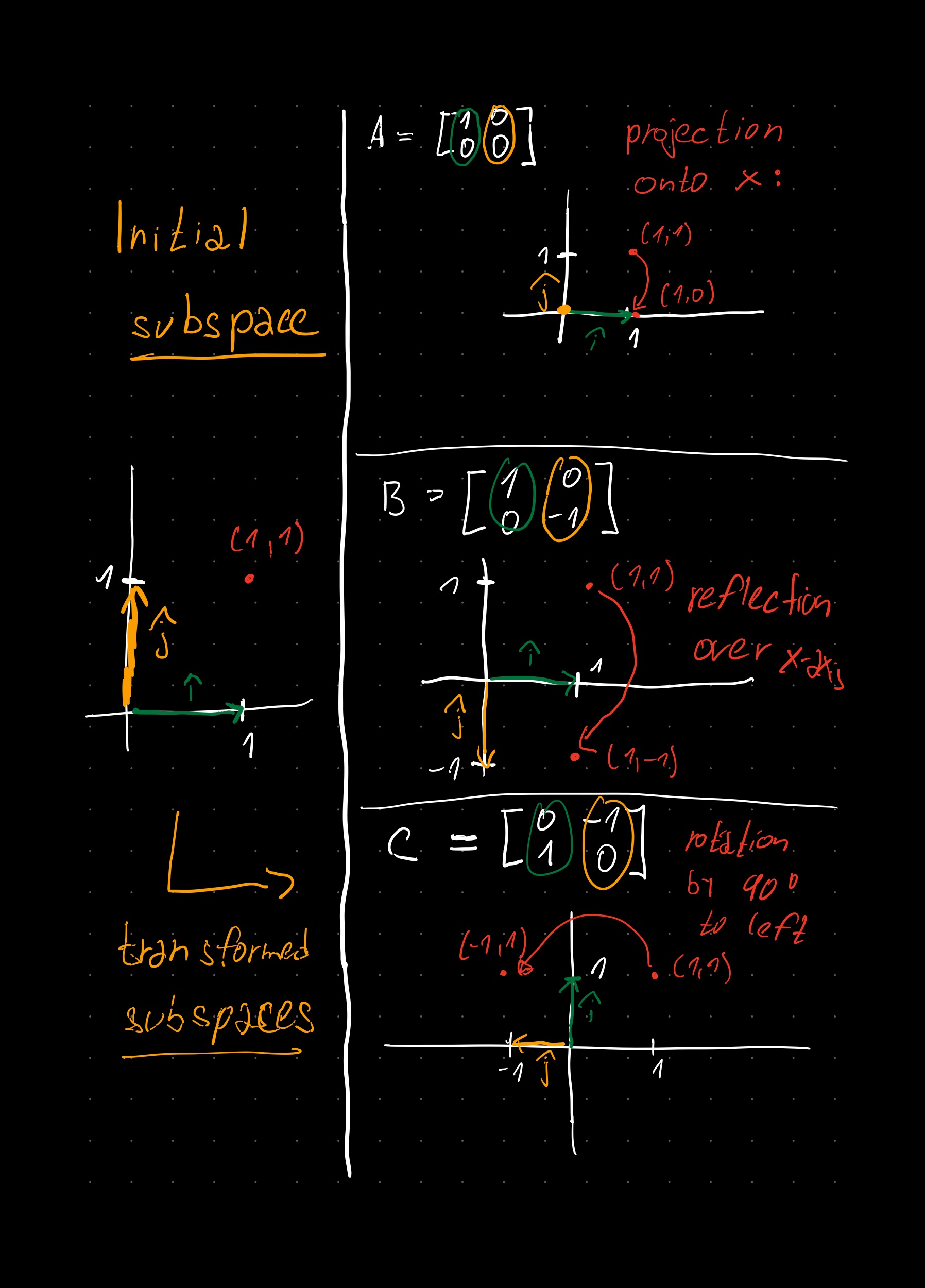
\[A=\left[\begin{array}{ll} 1 & 0 \\ 0 & 0 \end{array}\right] \quad B=\left[\begin{array}{cc} 1 & 0 \\ 0 & -1 \end{array}\right] \quad C=\left[\begin{array}{cc} 0 & -1 \\ 1 & 0 \end{array}\right]\]consider the maps \(f: \mathbb{R}^2 \rightarrow \mathbb{R}^2\) defined as
\[f(x, y)=A\left[\begin{array}{l} x \\ y \end{array}\right] \quad g(x, y)=B\left[\begin{array}{l} x \\ y \end{array}\right] \quad h(x, y)=C\left[\begin{array}{l} x \\ y \end{array}\right]\](and similarly for \(B\) and \(C\)). Apply the function to a few different vectors in \(\mathbb{R}^2\) and draw the result. What do \(f, g\) and \(h\) do? You should recognise these as basic geometric operations.
Solution (based on Rasmus’ solution)
Below you can see my solution. In the left column, you have the initial subspace. Notice the position of the two vectors \(\hat{\textbf{i}}\) and \(\hat{\textbf{j}}\). Then in the right column you can see how they got transformed. This transformation can be read from the given matrices. All vectors (points) will then undergo the exact same transformation as \(\hat{\textbf{i}}\) and \(\hat{\textbf{j}}\). If time, watch first 5 videos (up until chapter 4) of 3blue1brown videos. He does an amazing job explaining the visual intuition behind transformations and how they are related to matrices.
🔸 Exercise 3
Exercise 3. Consider the matrices \(B, C\) and functions \(g, h\) of the previous exercise. Recall that the composite function \(h \circ g\) is defined as \((h \circ g)(x, y)=h(g(x, y))\). Give an explicit formula for \((h \circ g)(x, y)\) ( i.e., a formula that mentions \(x$ and\)y\(, but not\)h$ and \(g\) explicitly), and find a matrix \(D\) such that
\[(h \circ g)(x, y)=D\left[\begin{array}{l} x \\ y \end{array}\right]\]What is the relationship between \(B, C\) and \(D\)? Can you make a general claim generalising your observation? Do the same for \(g \circ h\). Is there a geometric reason for why \(g \circ h \neq h \circ g\)?
Solution (based on Rasmus’ solution)
Each of the matrices represents a linear transformation. If we multiply the two matrices \(B, C\) we obtain a new matrix \(D\) that embedds transformation of the two matrices together. Therefore applying matrix \(D\) onto \(x\) alone is the same as applying \(B, C\) consecutively onto \(x\). Therefore, if we apply \((h \circ g)(x, y)\) this corresponds to \(D = CB\), conversely, if we apply \((g \circ h)(x, y)\) it translates into \(D = BC\). Therefore, if you use these matrices onto \(x\), you obtain \((y, x)\) and \((-y, -x)\). The geometric reasoning is that reflecting first and then rotating is not the same as rotating and then reflecting. This is why order matters when it comes to matrix multiplication.
🔸 Exercise 4
Construct a matrix \(A\) such that
\[A\left[\begin{array}{l} x \\ y \\ z \end{array}\right]=x u+y v+z w\]for any \(x, y, z\) where
\[u=\left[\begin{array}{l} 1 \\ 2 \\ 3 \end{array}\right] \quad v=\left[\begin{array}{l} 2 \\ 1 \\ 0 \end{array}\right] \quad w=\left[\begin{array}{c} 0 \\ -1 \\ 2 \end{array}\right]\]Describe in words what \(A\) is:
\[A\left[\begin{array}{ll} x & r \\ y & s \\ z & t \end{array}\right]\]Solution (based on Rasmus’ solution)
First, \(A\) is a \(3 \times 3\) matrix whose columns are \(u, v, w\) respectively. Why? Try to do the actual matrix multiplication \(Ax\) where \(x\) is the \(3 \times 1\) column vector. If you watched 3blue1brown videos on this topic, you should notice that \(u, v, w\) are basis of the new subspace which is created by the transformation that the matrix \(A\) represents. Then the column vector \(x\) is a vector from the original subspace with the standard basis \(\hat{\textbf{i}}\), \(\hat{\textbf{j}}\) and \(\hat{\textbf{z}}\) that you want to map to the new transformed subspace. This is done trough multiplying each dimension of the column vector \(x\) by a corresponding basis vector in the new subspace. Now, if we think about the last question, on the left side we have linear transformation matrix \(A\) and on the right side we have \(3 \times 2\) matrix where each column represents vector from the original subspace. If we do the product of these two matrices, we obtain a new \(3 \times 2\) matrix where each column represents the transformed vectors. To summarize, this exercise aims to give you another perspective on matrix multiplication, specifically what it actually represents.
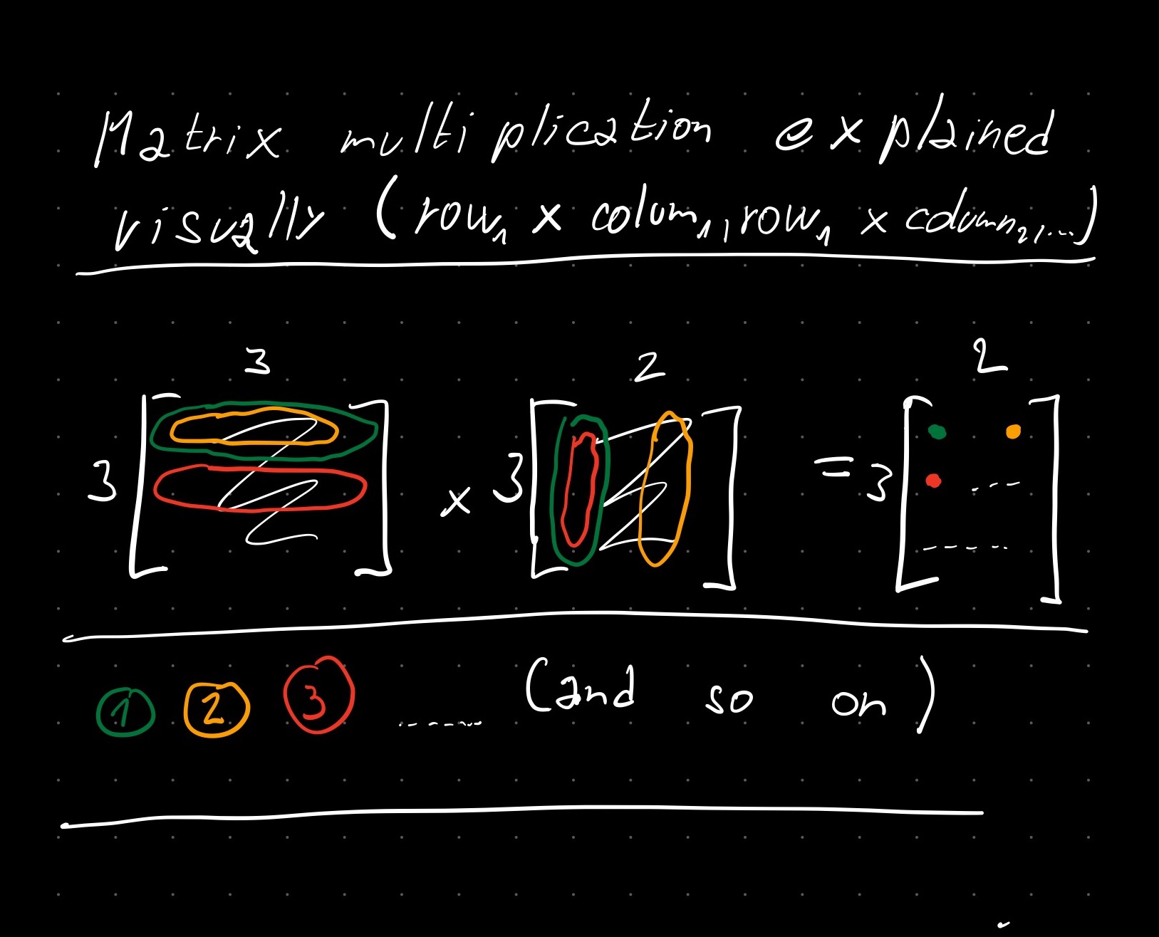
Below, I tried to show you how you can easily remember matrix multplication. First, determine what is the size of the output matrix. Then do a dot product between first row (left matrix) and first column (right matrix), then again first row and second column - continue until you fill the first row of the output matrix. Then start filling second row by dot product between second row and first column, …
🔸 Exercise 5
Write the matrix
\[A=\left[\begin{array}{ll} 0 & 2 \\ 1 & 0 \end{array}\right]\]as a product of elementary matrices, find the inverses to those elementary matrices, and use that to find an inverse to \(A\). Check your result, and be careful about the order of multiplication.
Solution (based on Rasmus’ solution)
First of all, quick recap on elementary matrices, what are they? According to the book’s definition, elementary matrix is a square matrix (challenge: try to think why square) that was created by a single row operation from an identity matrix. Put in the context of the previous exercises, both types of matrices can be viewed as linear transformations. The special thing about identity matrix is that its transformation has essentially no effect. Natural question is why? Here is an example of a simple \(2 \times 2\) identity matrix:
Recall that each column represents basis of the transformed vector space. However, here we see that the columns actually represents basis of the original vector space. Nice, but how is this related to the elementry matrices? Well, each row operation that you apply to the identity matrix results in new basis, thus each row operation is some kind of transformation (e.g. rotation, …) If you keep applying new and new row operations, you are essentially applying new and new transformations. The end result is some matrix with the new basis which embeds all the applied transformations. The idea with elementary matrices is that they simply embed just one transformation. If you then multiply several elementary matrices together then you get to the matrix that embeds all these transformations. So how do we actually rewrite \(A\) as a product of elementary matrices? Well, from the first lecture you know how to obtain reduced row echelon form of a matrix which in case of a square matrix is the identity matrix, so you can start by doing that. In this case the operations are:
-
Row swap: \(R_1\) and \(R_2\)
-
Row multiplication: \(\frac{1}{2}R_2 \Rightarrow R_2\)
Therefore as a result, using the notion of elementary matrices we can write our process as follows:
\[E_2 E_1 A = I\]Problems is that we are interested in rewriting \(A\) as the product of elementary matrices, i.e., we need to separate A on the left, so:
\[\begin{aligned} E_1^{-1}E_2^{-1}E_2 E_1 A = IE_1^{-1}E_2^{-1} \end{aligned}\]From the book we now this can be done since elementary matrices are invertible and their inverse is also an elementary matrix. Therefore, as a result, we have:
\[\begin{aligned} A = E_1^{-1}E_2^{-1} \end{aligned}\]So the only last step is to find the corresponding inverses to the \(E_1, E_2\) respectively. Since these are only \(2 \times 2\) matrices, you can use closed formula, given some matrix \(E\):
\[\begin{aligned} &E=\left[\begin{array}{ll} a & b \\ c & d \end{array}\right] \end{aligned}\]Then:
\[\begin{aligned} &E^{-1}=\frac{1}{a d-b c}\left[\begin{array}{cc} d & -b \\ -c & a \end{array}\right] \end{aligned}\]And therefore as a result:
\[A=\left[\begin{array}{ll} 0 & 1 \\ 1 & 0 \end{array}\right]\left[\begin{array}{ll} 1 & 0 \\ 0 & 2 \end{array}\right]\]Now, if we want to find inverse of \(A\), we can look at the initial equation again:
\[E_2 E_1 A = I\]If we multiply both sides by \(A^{-1}\) from the right side (remember order does matter) then:
\[\begin{aligned} E_2 E_1 A A^{-1} = I A^{-1} \\ E_2 E_1 = A^{-1} \\ A^{-1} = E_2 E_1 \end{aligned}\]Recall that \(E_2, E_1\) represent \(R_2\) multiplication by one half and swap of the \(R_1, R_2\) respectively. Therefore, we can write:
\[A^{-1}=\left[\begin{array}{ll} 1 & 0 \\ 0 & \frac{1}{2} \end{array}\right]\left[\begin{array}{ll} 0 & 1 \\ 1 & 0 \end{array}\right]=\left[\begin{array}{ll} 0 & 1 \\ \frac{1}{2} & 0 \end{array}\right]\]🔸 Exercise 6
Rewrite the matrix
\[B=\left[\begin{array}{cc} 3 & -2 \\ 1 & 0 \end{array}\right]\]to the identity matrix by a sequence of elementary row operations. Use this information to write \(B\) as a product of elementary matrices and use this to compute the inverse of \(B\).
Solution (based on Rasmus’ solution)
This exercise is pretty much the same as the previous one. The essential equation from which everything follows is:
\[E_k \dots E_1 B = I\]This shows that using \(k\) row operations, we turned \(B\) into an identity matrix. Notice the order of \(E\), i.e., we apply the operations from left to \(B\). We have two tasks:
(a) Write \(B\) as product of elementary matrices
(b) Find inverse of \(B\) (for that we can use some work from (a))
The first task can be broken down into:
- Finding the row operations that will turn \(B\) into an identity matrix:
- These operations correspond to the following matrices:
- Then realizing that \(B = E_1^{-1} \dots E_k^{-1}\), thus finding corresponding inverses to the operations from the first step (3 operations, 3 elementary matrices):
Finally, (b) can be completed by realizing that \(B^{-1} = E_k \dots E_1\). This means just plugging the elementary matrices from step 2 into this equation:
\[B^{-1}=E_3E_2E_1=\left[\begin{array}{cc} 1 & 0 \\ 0 & -\frac{1}{2} \end{array}\right]\left[\begin{array}{cc} 1 & 0 \\ -3 & 1 \end{array}\right]\left[\begin{array}{ll} 0 & 1 \\ 1 & 0 \end{array}\right]=\left[\begin{array}{cc} 1 & 0 \\ 0 & -\frac{1}{2} \end{array}\right]\left[\begin{array}{cc} 0 & 1 \\ 1 & -3 \end{array}\right]=\left[\begin{array}{cc} 0 & 1 \\ -\frac{1}{2} & \frac{3}{2} \end{array}\right]\]Exercises from book
⛑ Exercise 2.3.66
Prove that if \(A^2 = A\) then:
\[I - 2A = (I - 2A)^{-1}\]Solution
If we were to write the above formally using the notation from last week:
\[A^2 = A \Longrightarrow (I - 2A)^{-1}\]My goal will be to modify the right side so we get the left side. Let’s start by introducing a substitution:
\[B = I - 2A\]Then we can write:
\[\begin{aligned} B = B^{-1} \\ BB = B^{-1}B \\ B^2 = I \\ B^2 - I = 0 \end{aligned}\]Recall the known formula \(x^2 - 1 = (x + 1)(x - 1)\), using it, we can write:
\[\begin{aligned} B^2 - I = 0 \\ (B + I)(B - I) = 0 \\ \end{aligned}\]If we now substitute back:
\[\begin{aligned} (B + I)(B - I) = 0 \\ (I - 2A + I)(I - 2A - I) = 0 \\ (2I - 2A)(-2A) = 0 \\ -4A + 4A^2 = 0 \\ 4A^2 = 4A \\ A^2 = A \end{aligned}\]This means:
\[A^2 = A \Longrightarrow A^2 = A\]which is of course true.
🔍 About the page
- Last updated: 07/09/2022
- Unless othewise stated, exercises come from the book:
Elementary Linear Algebra, International Metric Edition, Ron Larson - Purpose: This page was created as part of a preparation for my teaching assistant session in the course Linear algebra and optimization managed by
Rasmus Ejlers Møgelberg. Please note that unless othewise stated, the solutions on this page are my own, thus it should not be considered as official solutions provided as part of the course.